Home » Sentiment Analysis On E-Commerce Dataset Example

Sentiment Analysis On E-Commerce Dataset Example

We’re going to apply sentiment analysis on an e-commerce dataset and solve a simple binary classification example.

Furthermore, we’re going to use a model architecture with LSTM and fully connected layers using Tensorflow machine learning library.

In order to label our dataset samples into 2 possible classes, we’ll use some of the features from pandas library. Additionally, we’ll use review score data to set each sample a negative or a positive label.

About the dataset

We’re going to be working with a public Brazilian e-commerce dataset of orders from Olist Store. Moreover, it contains information of 100k orders from 2016 to 2018.

Furthermore, this dataset includes multiple csv files, each containing different kind of data of an order. Since we’ll be doing sentiment analysis on review orders, we’ll use order reviews csv file.

Sentiment analysis example with python

First of all, we’ll need to import all the necessary libraries, before we start working with our dataset.

import pandas as pd
import numpy as np
import tensorflow as tf
from sklearn.model_selection import train_test_split
from kaggle.api.kaggle_api_extended import KaggleApi

Next, we’ll need to authenticate the connection with Kaggles API, so we’ll be able to download the dataset files. To clarify, this step is only necessary if you want to download the dataset from within the script.

And after we do this, we can call APIs function to go ahead and download our dataset.

api = KaggleApi()
api.authenticate()

api.dataset_download_files(
    'olistbr/brazilian-ecommerce',
    path='datasets/brazilian e-commerce',
    unzip=True
)

Okay, now we’re ready to store the contents of order reviews csv file into a pandas dataframe.

data_dir = 'datasets/brazilian e-commerce/olist_order_reviews_dataset.csv'
data = pd.read_csv(data_dir)
print(data.head())

Next we’re going to set some hyperparameters, we’ll be using in the data preprocessing section and neural network training.

RANDOM_STATE = 42
TRAIN_SPLIT = 0.8
OOV_TOK = '<OOV>'
VOCAB_SIZE = 10000
EMBEDDING_DIM = 16
MAX_LENGTH = 120
BATCH_SIZE = 128
EPOCHS = 25
EARLY_STOPPING_CRITERIA = 3
DROPOUT_P = 0.4
LEARNING_RATE = 0.01
MOMENTUM = 0.9
MAX_ITER = 10000
N_JOBS = 4

Okay, now we’re ready for the data preprocessing part of this project. Futhermore, we’re going to define a function, in which we’ll do everything to prepare the data for training.

def preprocess_data(data):

    # get message and review score column
    text_col = 'review_comment_message'
    score_col = 'review_score'

    # remove rows with missing messages
    data.dropna(subset=[text_col], inplace=True)

    # create a column with labels belonging to 2 classes
    data['label'] = pd.cut(data[score_col], bins=[0, 2, 5], labels=[0, 1])

    # discard unnecessary columns
    data = data[[text_col, 'label']]
    print(data)

    # split data into training and testing subsets
    X_train, X_test, y_train, y_test = train_test_split(
        data[text_col], data['label'],
        train_size=TRAIN_SPLIT,
        random_state=RANDOM_STATE
    )

    # tokenize text data
    tokenizer = tf.keras.preprocessing.text.Tokenizer(num_words=VOCAB_SIZE, oov_token=OOV_TOK)
    tokenizer.fit_on_texts(X_train)

    # pad text data
    def pad_data(data):
        sequences = tokenizer.texts_to_sequences(data)
        padded = tf.keras.preprocessing.sequence.pad_sequences(
            sequences, maxlen=MAX_LENGTH, truncating='post'
        )
        return padded
    
    X_train = pad_data(X_train)
    X_test = pad_data(X_test)

    return X_train, X_test, y_train, y_test

X_train, X_test, y_train, y_test = preprocess_data(data)

And now finally, all we need to do is create a model, compile it, train it, and evaluate it. To clarify, this is the standard procedure for training machine learning models, in case if it sounds a little overwhelming.

We’re also going to set up an early stopping callback, which will stop the training process, once the model stops improving on validation data.

def create_model():

    input = tf.keras.Input(shape=(MAX_LENGTH))

    x = tf.keras.layers.Embedding(VOCAB_SIZE, EMBEDDING_DIM, input_length=MAX_LENGTH)(input)
    x = tf.keras.layers.LSTM(32, return_sequences=True)(x)
    x = tf.keras.layers.LSTM(32)(x)
    x = tf.keras.layers.Dropout(DROPOUT_P)(x)

    x = tf.keras.layers.Dense(800, activation='relu')(x)
    x = tf.keras.layers.Dropout(DROPOUT_P)(x)
    x = tf.keras.layers.Dense(400, activation='relu')(x)
    x = tf.keras.layers.Dropout(DROPOUT_P)(x)
    
    output = tf.keras.layers.Dense(1, activation='sigmoid')(x)

    model = tf.keras.Model(input, output)

    return model

earlyStoppingCallback = tf.keras.callbacks.EarlyStopping(
    monitor='val_loss',
    patience=EARLY_STOPPING_CRITERIA,
    verbose=1,
    restore_best_weights=True
)

model = create_model()

model.compile(
    loss=tf.keras.losses.BinaryCrossentropy(),
    optimizer=tf.keras.optimizers.SGD(learning_rate=LEARNING_RATE, momentum=MOMENTUM),
    metrics=['accuracy']
)

print(model.summary())

history = model.fit(
    x=X_train,
    y=y_train,
    validation_data=(X_test, y_test),
    epochs=EPOCHS,
    batch_size=BATCH_SIZE,
    callbacks=[earlyStoppingCallback]
)

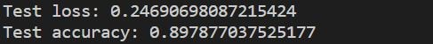
test_loss, test_acc = model.evaluate(X_test, y_test)
print("Test loss:", test_loss)
print("Test accuracy:", test_acc)

After we evaluate the model, we also print out the final results, being the loss and accuracy of the model.

Conclusion

To conclude, we solved a simple binary classification problem using LSTM and fully connected layers. Furthermore, this is a classic example of natural language processing problem, where we can show how easy, but powerful it can be.

I hope you gained a better understanding about the implementation of sentiment analysis in natural language processing by following this example.