
Example of Classifying 3D Figures With Tensorflow
In this post, we’ll be making a simple algorithm for classifying 3D figures using Conv3D layers from Tensorflow. Furthermore, we’ll be working with 3D MNIST dataset, which is available on Kaggle. Therefore, we’re also going to use the Kaggle API to download it.
As you’ll be able to see, these types of networks are not all that different from classic convolutional neural networks we use to classify images. Main difference lies in the data preprocessing part, because we’re dealing with 3D objects.
Prerequisites
As it is with every other python project we tackle, first thing we need to do is import all the necessary libraries and tools.
import tensorflow as tf
import numpy as np
from matplotlib.cm import ScalarMappable
import matplotlib.pyplot as plt
import h5py
import os
from kaggle.api.kaggle_api_extended import KaggleApi
Pretty standard, as it goes with any other machine learning example. However, for this one we’ll also need the h5py library for loading in the dataset which is in .h5 format.
Next thing we need to do is authenticate connection with Kaggle using their API, so we can download the data. After this is done, we can also go ahead and download the dataset files.
api = KaggleApi()
api.authenticate()

ROOT = os.path.dirname(__file__)

api.dataset_download_files(
    'daavoo/3d-mnist',
    path=os.path.join(ROOT, 'data'),
    unzip=True
)
Before, we get into data preprocessing, I’d like to set a few hyperparameters first. Reason for this is so whenever I’m experimenting and changing them, they’re close to the start of the script.
# hyperparameters
BATCH_SIZE = 128
EPOCHS = 100
CLASSES = 10
Data preprocessing
Now we’re ready for one of the most crucial steps in this whole process, which is preparing the data. In order to load in the data for this particular example, we’ll need to define a couple of functions.
Basically, the following functions will handle the conversion of each data sample into numpy array of correct shape.
def array_to_color(array, cmap='Oranges'):
    s_m = ScalarMappable(cmap=cmap)
    return s_m.to_rgba(array)[:,:-1]

def rgb_data_transform(data):
    data_t = []
    for i in range(data.shape[0]):
        data_t.append(array_to_color(data[i]).reshape(16, 16, 16, 3))
    return np.asarray(data_t, dtype=np.float32)
At this stage, we’re ready to read the dataset file and get the data in the right format to start training our model.
with h5py.File(os.path.join(ROOT, 'data', 'full_dataset_vectors.h5'), 'r') as hf:
    X_train = hf['X_train'][:]
    y_train = hf['y_train'][:]
    X_test = hf['X_test'][:]
    y_test = hf['y_test'][:]

    sample_shape = (16, 16, 16, 3)
    X_train = rgb_data_transform(X_train)
    X_test = rgb_data_transform(X_test)

    y_train = tf.keras.utils.to_categorical(y_train).astype(np.integer)
    y_test = tf.keras.utils.to_categorical(y_test).astype(np.integer)
Defining & training the model for classifying 3D figures
We’re finally ready to setup our model and train it on the data we just prepared. Furthemore, the special thing about this model is that we’ll be using Conv3D layers.
However, you must keep in mind that training such models will be computationally more expensive. Perhaps, this example might not show that, but when working with real world examples, adding each dimension to your data samples can have a significant impact on computational cost.
So, without further a do, let’s define the architecture of our model.
model = tf.keras.Sequential([
    tf.keras.layers.Conv3D(32, kernel_size=(3, 3, 3), activation='relu', kernel_initializer='he_uniform', input_shape=sample_shape),
    tf.keras.layers.MaxPooling3D(pool_size=(2, 2, 2)),
    tf.keras.layers.Dropout(0.6),
    tf.keras.layers.Conv3D(64, kernel_size=(3, 3, 3), activation='relu', kernel_initializer='he_uniform'),
    tf.keras.layers.MaxPooling3D(pool_size=(2, 2, 2)),
    tf.keras.layers.Dropout(0.6),
    tf.keras.layers.Flatten(),
    tf.keras.layers.Dense(256, activation='relu', kernel_initializer='he_uniform'),
    tf.keras.layers.Dense(CLASSES, activation='softmax')
])

print(model.summary())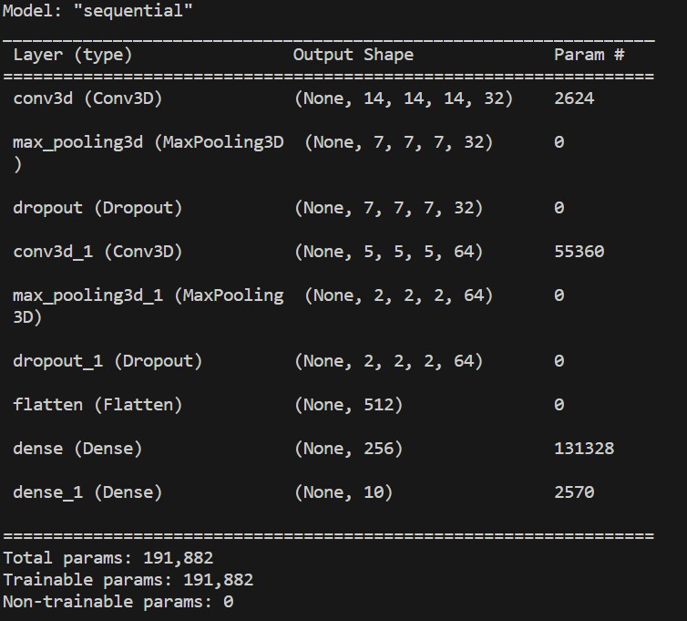
Okay, we’re ready to compile it now. We’ll use Adam optimizer, categorical crossentropy loss function, and also throw in accuracy metric.
model.compile(loss=tf.keras.losses.categorical_crossentropy,
              optimizer='adam', metrics=['accuracy'])
The following part of this process is the one we’ve been all waiting for, which is training the model. Before we send it, we’ll also use a couple of callbacks to prevent wasting resources.
We’ll use model checkpoint callback, which will save model weights at the end of each epoch. Another callback we’ll use is early stopping callback, which will check whether the model keeps improving each epoch and once it stops doing so, it will prematurely stop the training process.
callbacks = [
    tf.keras.callbacks.ModelCheckpoint(
        filepath=os.path.join(ROOT, 'training_checkpoints', 'ckpt_{epoch}'),
        save_weights_only=True),
    tf.keras.callbacks.EarlyStopping(
        monitor='val_loss',
        patience=5,
        verbose=1,
        restore_best_weights=True),
]

history = model.fit(X_train, y_train,
                    batch_size=BATCH_SIZE,
                    epochs=EPOCHS,
                    verbose=1,
                    validation_split=0.2,
                    callbacks=callbacks)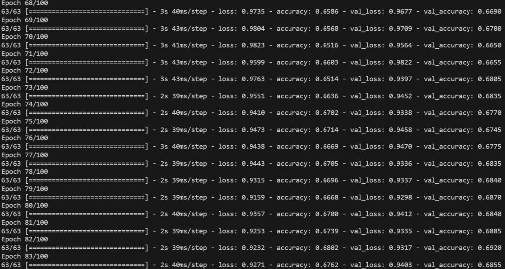
Evaluating the trained model
Once the training process finishes, we can evaluate its performance by testing it on the test set of the dataset. Furthermore, we’ll plot the loss and accuracy data from each epoch.
# getting results
score = model.evaluate(X_test, y_test, verbose=1)
print(f'Test loss: {score[0]} / Test accuracy: {score[1]}')
plt.plot(history.history['loss'], label='Categorical crossentropy (training data)')
plt.plot(history.history['val_loss'], label='Categorical crossentropy (validation data)')
plt.plot(history.history['accuracy'], label='Accuracy (training data)')
plt.plot(history.history['val_accuracy'], label='Accuracy (validation data)')
plt.title('Model performance for 3D MNIST Keras Conv3D example')
plt.ylabel('Loss value')
plt.xlabel('No. epoch')
plt.legend(loc="upper left")
plt.show()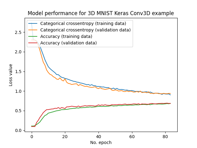
Conclusion
We made a simple example using Conv3D layers in a model for classifying 3D figures. I hope you gained a better understanding about how it works as I did while working on this project.