Home » Machine Learning » How To Make Variational Autoencoder With Tensorflow

How To Make Variational Autoencoder With Tensorflow

In this post, we’ll demonstrate how to make a simple variational autoencoder model using Tensorflow. Furthermore, we’ll be working with MNIST dataset of handwritten digits, so we don’t need to do much preprocessing.

This type of models might seem super complicated at first glance. But as you’ll see further in this tutorial, there isn’t all that much to them. Additionally, there is already a tutorial about them on official Tensorflow website. However, I just feel they overcomplicated things and made it less clear to understand how it all works.

Prerequisites

Before we begin, we’ll need to import all the necessary libraries and tools for this project. These include Tensorflow, which is the main library of this project, Numpy, and Matplotlib.

We’ll also need to disable eager execution, since Tensorflow tends to throw errors with the loss function we’re about to use.

import tensorflow as tf
import numpy as np
import matplotlib.pyplot as plt
import os

from tensorflow.python.framework.ops import disable_eager_execution
disable_eager_execution()

Getting data ready

Next step in this whole process is to load in the MNIST dataset. Luckily, it is readily available among Keras datasets, which we can load in a single line.

However, we’ll need to take a couple extra steps to get it completely ready for training the variational autoencoder. We’ll also set a couple of hyperparameters for it in this step as well.

(input_train, target_train), (input_test, target_test) = tf.keras.datasets.mnist.load_data()

img_width, img_height = input_train.shape[1], input_train.shape[2]
batch_size = 128
epochs = 100
latent_dim = 2

input_train = input_train.reshape(input_train.shape[0], img_height, img_width, 1)
input_test = input_test.reshape(input_test.shape[0], img_height, img_width, 1)
input_shape = (img_height, img_width, 1)

input_train = input_train.astype('float32')
input_test = input_test.astype('float32')

input_train /= 255
input_test /= 255

To explain what is actually going on here, we changed the shape of imported dataset to give each image 3 dimensions, convert the values into type float, and normalize the values, bringing them into range between 0 and 1.

Making the variational autoencoder model

Now, we’re ready to start making the variational autoencoder model. But before, we get into coding, I should explain how it works.

The whole model is actually made up of 2 models, encoder and decoder. Additionally, its architecture resembles an hourglass, where encoder compresses data into a latent space and decoder reconstructs it back.

To clarify, latent space is the bottleneck part of the autoencoder, where data is represented in just a couple of dimensions.

So, without further a do, let’s make the encoder.

# Encoder
inp = tf.keras.layers.Input(shape=input_shape, name='encoder_input')
cx = tf.keras.layers.Conv2D(filters=32, kernel_size=3, strides=2, padding='same', activation='relu')(inp)
cx = tf.keras.layers.BatchNormalization()(cx)
cx = tf.keras.layers.Conv2D(filters=64, kernel_size=3, strides=2, padding='same', activation='relu')(cx)
cx = tf.keras.layers.BatchNormalization()(cx)
x = tf.keras.layers.Flatten()(cx)
x = tf.keras.layers.Dense(20, activation='relu')(x)
x = tf.keras.layers.BatchNormalization()(x)
mu = tf.keras.layers.Dense(latent_dim, name='latent_mu')(x)
sigma = tf.keras.layers.Dense(latent_dim, name='latent_sigma')(x)

def sample_z(args):
    mu, sigma = args
    batch = tf.shape(mu)[0]
    dim = mu.shape[1]
    eps = tf.random.normal(shape=(batch, dim))
    return mu + tf.exp(sigma / 2) * eps

z = tf.keras.layers.Lambda(sample_z, output_shape=(latent_dim, ), name='z')([mu, sigma])

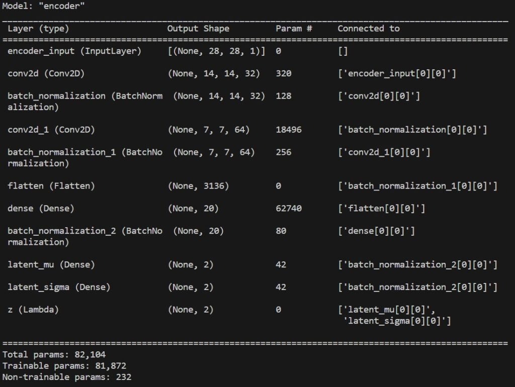
encoder = tf.keras.Model(inp, [mu, sigma, z], name='encoder')
print(encoder.summary())

Okay, now we need to make the decoder. We also need to keep in mind that it’s important to make encoder and decoder symmetrical.

conv_shape = cx.shape

# Decoder
d_inp = tf.keras.layers.Input(shape=(latent_dim, ), name='decoder_input')
x = tf.keras.layers.Dense(conv_shape[1] * conv_shape[2] * conv_shape[3], activation='relu')(d_inp)
x = tf.keras.layers.BatchNormalization()(x)
x = tf.keras.layers.Reshape((conv_shape[1], conv_shape[2], conv_shape[3]))(x)
cx = tf.keras.layers.Conv2DTranspose(filters=64, kernel_size=3, strides=2, padding='same', activation='relu')(x)
cx = tf.keras.layers.BatchNormalization()(cx)
cx = tf.keras.layers.Conv2DTranspose(filters=32, kernel_size=3, strides=2, padding='same', activation='relu')(cx)
cx = tf.keras.layers.BatchNormalization()(cx)
out = tf.keras.layers.Conv2DTranspose(filters=1, kernel_size=3, strides=1, activation='sigmoid', padding='same', name='decoder_output')(cx)

decoder = tf.keras.Model(d_inp, out, name='decoder')
print(decoder.summary())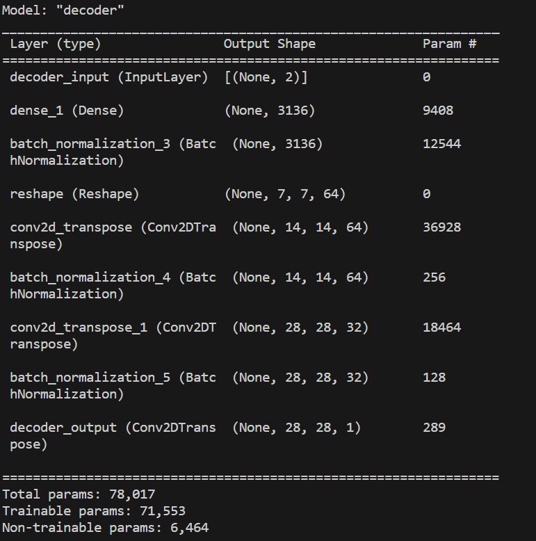

For the purpose of making things symmetrical, we used the shape dimensions of last convolutional layer in the encoder. We also set the same amount of filters in convolutional layers, but in reverse order.

Now, we have all the parts we need to put together the variational autoencoder model.

# VAE
vae_outputs = decoder(encoder(inp)[2])
vae = tf.keras.Model(inp, vae_outputs, name='vae')
print(vae.summary())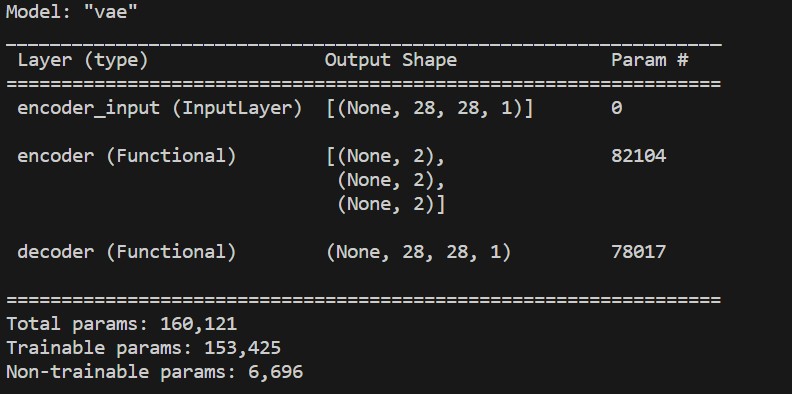

As we can see the dimensions in the input and output match, which is a great sign we did everything right so far.

Training the variational autoencoder model

Before we can start training the model, we need to compile it first. However, there’s a catch, we need to use a custom loss function for this to work properly.

So let’s define the loss function first.

def kl_reconstruction_loss(true, pred):
    reconstruction_loss = tf.keras.losses.binary_crossentropy(tf.keras.backend.flatten(true), tf.keras.backend.flatten(pred)) * (img_width * img_height)
    kl_loss = 1 + sigma - tf.math.square(mu) - tf.math.exp(sigma)
    kl_loss = tf.math.reduce_sum(kl_loss, axis=-1)
    kl_loss *= -0.5

    return tf.math.reduce_mean(reconstruction_loss + kl_loss)

Okay, now we’re ready to compile the model.

vae.compile(optimizer='adam', loss=kl_reconstruction_loss)

Following part is what we’ve been waiting for this whole time. Now it’s time to train the model. We’re also going to use a couple of callbacks, for saving weights and checking if the model is still improving every epoch.

callbacks = [
    tf.keras.callbacks.ModelCheckpoint(
        filepath=os.path.join(os.path.dirname(__file__), 'training_checkpoints', 'ckpt_{epoch}'),
        save_weights_only=True),
    tf.keras.callbacks.EarlyStopping(
        monitor='loss',
        patience=5,
        verbose=1,
        restore_best_weights=True),
]

vae.fit(input_train, input_train, epochs=epochs, batch_size=batch_size, validation_split=0.2, callbacks=callbacks)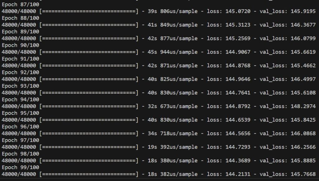

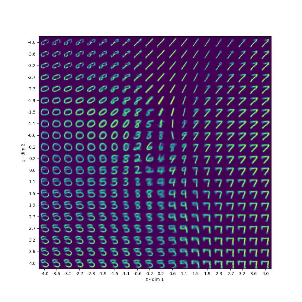
Plotting from latent space

For the final part of this tutorial, we’ll plot samples from latent space, where we’ll get the decoder to generate from latent space values.

def plot_decoded(decoder):
    num_samples = 20
    figure = np.zeros((img_width * num_samples, img_height * num_samples, 1))
    grid_x = np.linspace(-4, 4, num_samples)
    grid_y = np.linspace(-4, 4, num_samples)

    for i, yi in enumerate(grid_y):
        for j, xi in enumerate(grid_x):
            z_sample = np.array([[xi, yi]])
            x_decoded = decoder.predict(z_sample)
            digit = x_decoded[0].reshape(img_width, img_height, 1)
            figure[i * img_width: (i + 1) * img_width,
                   j * img_height: (j + 1) * img_height] = digit
    plt.figure(figsize=(10, 10))
    start_range = img_width // 2
    end_range = num_samples * img_width + start_range
    pixel_range = np.arange(start_range, end_range, img_width)
    sample_range_x = np.round(grid_x, 1)
    sample_range_y = np.round(grid_y, 1)
    plt.xticks(pixel_range, sample_range_x)
    plt.yticks(pixel_range, sample_range_y)
    plt.xlabel('z - dim 1')
    plt.ylabel('z - dim 2')

    fig_shape = np.shape(figure)
    if fig_shape[2] == 1:
        figure = figure.reshape((fig_shape[0], fig_shape[1]))
    plt.imshow(figure)
    plt.show()

plot_decoded(decoder)

And the following image is what we get from it.