Data Visualization & Training Regression Model Using LazyPredict
In this post, we’ll use a movie dataset to train a regression model for predicting gross values utilizing lazypredict package. Furthermore, we’re going to use pandas package for wrangling data and matplotlib for visualizing it.
In order to find the optimal model architecture or type, we’re going to utilize lazypredict. To clarify, this package allows us to test our dataset on multiple different model architectures. Additionally, resulting output shows us performance insight for each model.
In our case, we’ll be working with regression, which mean that we’ll need to use LazyRegressor class from this package.
Setting up prerequisites
First of all, you’ll need to install the packages we’ll need for this project. While scikit-learn package is quite common and you probably already have it, chances are that you’ll have to install lazypredict as it’s less known. Furthermore, you can install both packages with the following commands.
pip install -U scikit-learn
pip install lazypredict
We’re also going to utilize Kaggle’s API with a python package, which will allow us to download the dataset right from the code. If you’re not familiar with it yet, I’d recommend you check out a post about setting up Kaggle API and downloading datasets.
Next thing we need to do is create a Python file and import all the necessary libraries. This is a standard part of every Python project.
# Import necessary libraries
import os
import pandas as pd
import matplotlib.pyplot as plt
from sklearn.model_selection import train_test_split
from lazypredict.Supervised import LazyRegressor
from kaggle.api.kaggle_api_extended import KaggleApi
import lightgbm as lgb
Alright, now we’re ready to download the dataset. Before we can call the Kaggle API, we’ll need to authenticate the connection with it first. After, we can download the dataset and import its contents in our code.
# Authenticate connection with Kaggle API
api = KaggleApi()
api.authenticate()

# Download the dataset
ROOT = os.path.dirname(__file__)
data_path = os.path.join(ROOT, 'Most Profitable Movies of All Time - Top 500 Movies.csv')
api.dataset_download_file(
    'joebeachcapital/top-500-hollywood-movies-of-all-time',
    file_name='Most Profitable Movies of All Time - Top 500 Movies.csv',
    path=ROOT
)

# Load the dataset
movies = pd.read_csv(data_path)
Next, we’ll clean the dataset a little, which includes removing a couple of columns and setting the titles as indexes. The reason for this is, because title is unique for each data point (row).
# Clean up dataset
movies.drop([
    'source',
    'budget source',
    'force label'
    ], axis=1, inplace=True)
movies.set_index('title ', inplace=True)
movies['horror'] = movies['horror'].str.lower()

print(movies.head())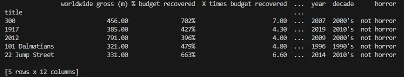
Visualizing data for each decade
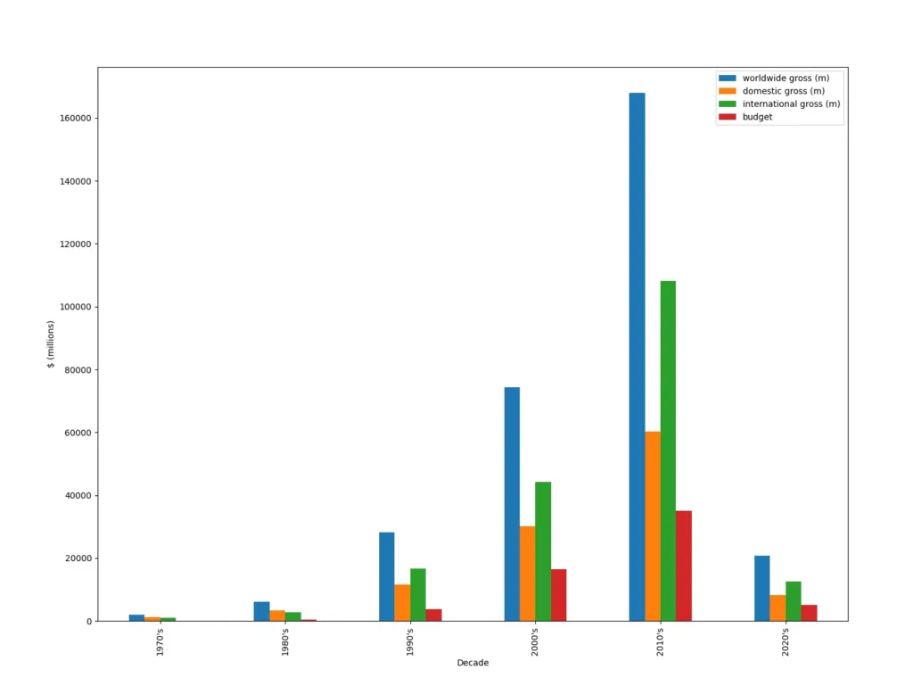
Before we can plot the data for each decade, we’ll need to create a new dataframe from the dataset. Furthermore, we’ll need to extract the budget and gross information, which we’ll sum up for each decade and plot it.
sums = {}
for decade in set(movies['decade']):
    movies_by_decade = movies.loc[movies['decade'] == decade]
    sums[decade] = {
        'worldwide gross (m)': movies_by_decade['worldwide gross (m)'].sum(),
        'domestic gross (m)': movies_by_decade['domestic gross (m)'].sum(),
        'international gross (m)': movies_by_decade['international gross (m)'].sum(),
        'budget': movies_by_decade['budget  (millions)'].sum()
    }

sums = pd.DataFrame(sums)
sums = sums.reindex(columns=sorted(sums.columns))
sums = sums.T
print(sums)

sums.plot(
    xlabel='Decade',
    ylabel='$ (millions)',
    y=['worldwide gross (m)', 'domestic gross (m)', 'international gross (m)', 'budget'],
    kind='bar',
    figsize=(6, 4),
    use_index=True
)

plt.show()
The following graph shows the bar graph of the data we just created.
Using lazypredict to find the optimal model
In the following step, we’ll use the lazypredict library, which will train several different types of regression models to find which one performs the best. Furthermore, we’ll make a regression model for predicting the gross price for a given budget for the movie.
X = movies[['budget  (millions)']]
y = movies['worldwide gross']

X_train, X_test, y_train, y_test = train_test_split(
    X, y,
    train_size=0.8,
    random_state=42
)

reg = LazyRegressor(verbose=0, ignore_warnings=False, custom_metric=None)
models, predictions = reg.fit(X_train, X_test, y_train, y_test)

print(models)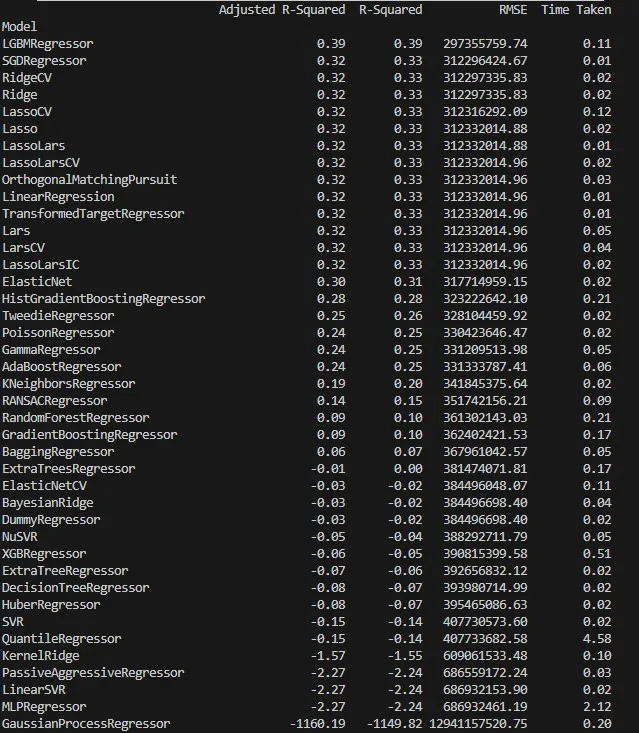
Okay, now that we know which type of model we should use for this problem, let’s train it. Additionally, we’ll make a pandas dataframe containing predictions and actual gross values, along with budgets and movie titles.
We’ll use this data for comparing the values and evaluating how good our model actually is.
param = {
    'metric': 'auc',
    'objective': 'regression'
}

train_data = lgb.Dataset(X_train, label=y_train)
model = lgb.train(param, train_data)

prediction = model.predict(X_test)
results = X_test

data = movies.loc[movies.index.isin(X_test.index), 'worldwide gross']
data = data.to_frame(name='worldwide gross')

data = data.sort_index(ascending=True)
data.reset_index(inplace=True)
results = results.sort_index(ascending=True)
results.reset_index(inplace=True)

results['Actual gross'] = data['worldwide gross']
results['Predictions'] = prediction
results.set_index('title ', inplace=True)
print(results)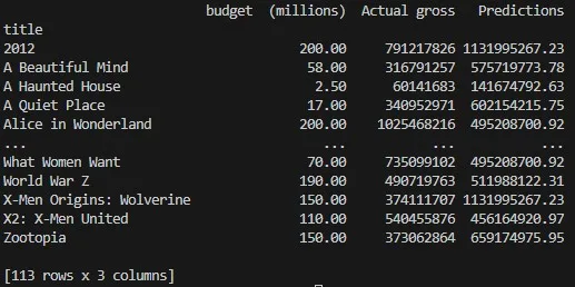
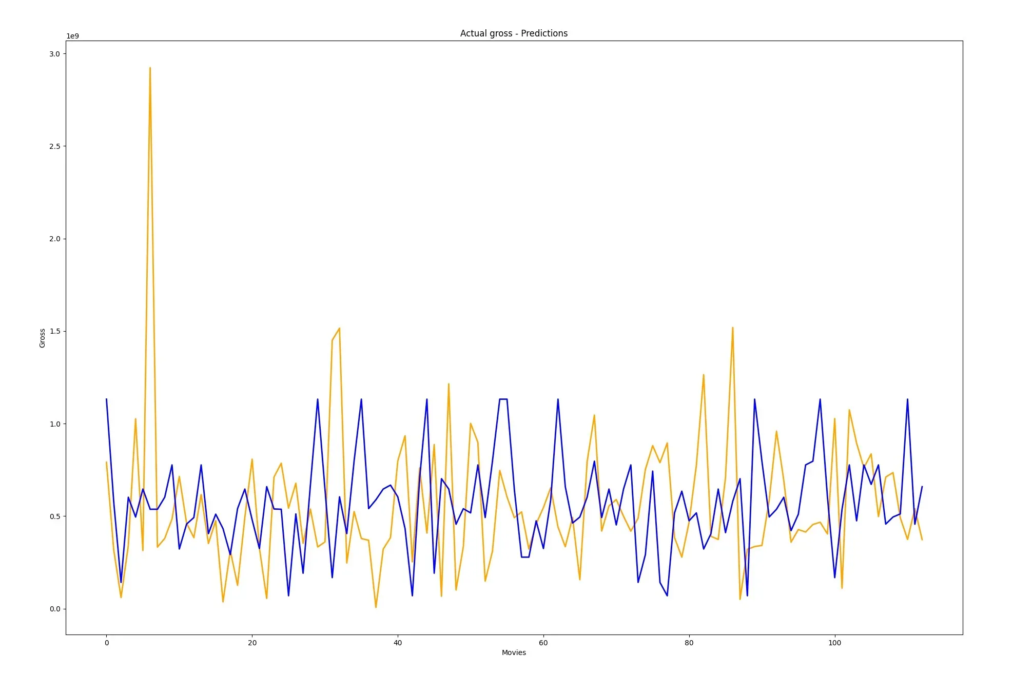
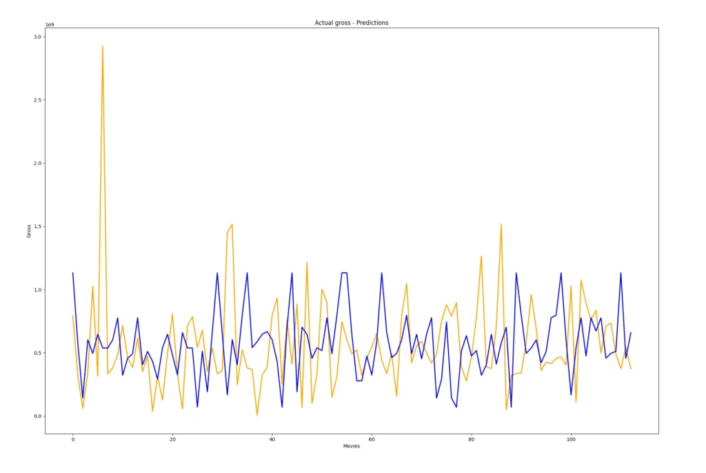
And for the final part of this guide, we’ll plot these value onto a graph.
Here is also the entire code of the project.
# Import necessary libraries
import os
import pandas as pd
import matplotlib.pyplot as plt
from sklearn.model_selection import train_test_split
from lazypredict.Supervised import LazyRegressor
from kaggle.api.kaggle_api_extended import KaggleApi
import lightgbm as lgb

# Authenticate connection with Kaggle API
api = KaggleApi()
api.authenticate()

# Download the dataset
ROOT = os.path.dirname(__file__)
data_path = os.path.join(ROOT, 'Most Profitable Movies of All Time - Top 500 Movies.csv')
api.dataset_download_file(
    'joebeachcapital/top-500-hollywood-movies-of-all-time',
    file_name='Most Profitable Movies of All Time - Top 500 Movies.csv',
    path=ROOT
)

# Load the dataset
movies = pd.read_csv(data_path)

# Clean up dataset
movies.drop([
    'source',
    'budget source',
    'force label'
    ], axis=1, inplace=True)
movies.set_index('title ', inplace=True)
movies['horror'] = movies['horror'].str.lower()

print(movies.head())

sums = {}
for decade in set(movies['decade']):
    movies_by_decade = movies.loc[movies['decade'] == decade]
    sums[decade] = {
        'worldwide gross (m)': movies_by_decade['worldwide gross (m)'].sum(),
        'domestic gross (m)': movies_by_decade['domestic gross (m)'].sum(),
        'international gross (m)': movies_by_decade['international gross (m)'].sum(),
        'budget': movies_by_decade['budget  (millions)'].sum()
    }

sums = pd.DataFrame(sums)
sums = sums.reindex(columns=sorted(sums.columns))
sums = sums.T
print(sums)

sums.plot(
    xlabel='Decade',
    ylabel='$ (millions)',
    y=['worldwide gross (m)', 'domestic gross (m)', 'international gross (m)', 'budget'],
    kind='bar',
    figsize=(6, 4),
    use_index=True
)

plt.show()

X = movies[['budget  (millions)']]
y = movies['worldwide gross']

X_train, X_test, y_train, y_test = train_test_split(
    X, y,
    train_size=0.8,
    random_state=42
)

reg = LazyRegressor(verbose=0, ignore_warnings=False, custom_metric=None)
models, predictions = reg.fit(X_train, X_test, y_train, y_test)

print(models)

param = {
    'metric': 'auc',
    'objective': 'regression'
}

train_data = lgb.Dataset(X_train, label=y_train)
model = lgb.train(param, train_data)

prediction = model.predict(X_test)
results = X_test

data = movies.loc[movies.index.isin(X_test.index), 'worldwide gross']
data = data.to_frame(name='worldwide gross')

data = data.sort_index(ascending=True)
data.reset_index(inplace=True)
results = results.sort_index(ascending=True)
results.reset_index(inplace=True)

results['Actual gross'] = data['worldwide gross']
results['Predictions'] = prediction
results.set_index('title ', inplace=True)
print(results)

tests = range(0, len(results))
fig, ax = plt.subplots(figsize=(12, 8))
ax.plot(tests, results['Actual gross'], label='Actual gross', color='orange', linewidth=2)
ax.plot(tests, results['Predictions'], label='Predictions', color='blue', linewidth=2)

plt.title('Actual gross - Predictions')
plt.xlabel('Movies')
plt.ylabel('Gross')
plt.show()
Conclusion
To conclude, we made a simple algorithm for finding optimal regression model using lazypredict library. Even more, we visualized data using matplotlib for plotting graphs. I learned a lot while working on this project, and I hope it proves itself helpful to you as well.