Polynomial Regression With Python Example
Polynomial regression is a type of regression analysis that models the relationship between a dependent variable and one or more independent variables as a polynomial function.
Furthermore, it extends the simple linear regression model by incorporating higher-degree terms of the independent variables. Therefore allowing for more complex relationships between the dependent and independent variables.
By doing so, it can capture nonlinear patterns in the data which linear regression would otherwise miss.
Brief comparison of polynomial regression with linear regression
Linear regression is a simple but popular method for modeling the relationship between a dependent variable and one or more independent variables.
Moreover, it assumes that the relationship is linear, meaning that we can represent it by a straight line.
However, in many real-world scenarios, the relationship between variables may be more complex and nonlinear.
Polynomial regression addresses this issue by including higher-degree terms of the independent variables, allowing the model to fit more complex, nonlinear relationships.
Although it can provide a better fit for certain datasets, it also increases the risk of overfitting. As a result of which the model becomes too complex and captures the noise in the data rather than the underlying pattern.
Importance of polynomial regression in machine learning and real-world applications
It’s an essential technique in machine learning and data analysis as it allows for the modeling of more complex relationships between variables.
Moreover, its flexibility in capturing nonlinear patterns makes it applicable to a wide range of real-world problems. For instance in forecasting, engineering, physics, economics, and environmental research.
In machine learning, we can use it as a standalone technique or in combination with other regression models to improve their predictive performance.
Additionally, it can serve as a basis for understanding more advanced machine learning algorithms. Some of which are also support vector machines and neural networks, which also aim to model complex relationships in data.
Mathematical foundation of polynomial regression
Linear regression and its limitations
Linear regression models the relationship between a dependent variable and one or more independent variables as a linear function.
While this simplicity can be advantageous in certain situations, it may not accurately capture more complex, nonlinear relationships that exist in real-world data.
Higher-order polynomial terms
Polynomial regression addresses this limitation by incorporating higher-order terms of the independent variables.
Furthermore, these terms allow the model to fit more complex relationships between the dependent and independent variables by adding curvature to the fitted function.
The polynomial regression model and its coefficients
We can express it as:
y = β0 + β1x + β2x^2 + ... + βnx^n + εwhere y is the dependent variable, x is the independent variable, n is the degree of the polynomial, βi are the coefficients to be estimated, and ε represents the error term.
Fitting a polynomial regression model
Fitting a polynomial regression model involves estimating the coefficients βi that minimize the sum of squared differences between the observed and predicted values of the dependent variable.
Moreover, we can do this by using various optimization techniques, such as gradient descent or least squares estimation.
Determining the appropriate polynomial degree
The risk of underfitting and overfitting
Choosing the appropriate polynomial degree is crucial in polynomial regression, as it determines the complexity of the model.
To clarify, a model with too low a degree may result in underfitting, where it fails to capture the underlying trend in the data.
Conversely, a model with too high a degree may result in overfitting, where it captures the noise in the data. Consequently leading to poor generalization to new data.
Model complexity and performance trade-offs
There is often a trade-off between model complexity and performance.
For instance, a more complex model may fit the training data better but may not generalize well to new data. Therefore, it’s essential to strike a balance between fitting the data and maintaining the model’s ability to generalize.
Cross-validation and model selection
Cross-validation is a popular technique for determining the appropriate polynomial degree.
Furthermore, it involves dividing the dataset into training and validation subsets. Where we fit models with different polynomial degrees on the training data, and evaluate their performance on the validation data.
Therefore, we can select the model with the best performance on the validation data as the final model.
Advantages and limitations of polynomial regression
Flexibility in modeling nonlinear relationships
Its primary advantage is its flexibility in modeling nonlinear relationships.
In order to fit complex data, where linear regression fails to, we can use polynomial regression. Reason for that are higher-degree terms that give it this sort of flexibility.
Interpretability and visualization of polynomial regression models
Polynomial regression models are generally easy to interpret and visualize, as they represent a smooth curve or surface.
This makes them useful for understanding relationships between variables and for communicating findings to non-technical audiences.
Limitations in extrapolation and the curse of dimensionality
Polynomial regression also has its limitations, such as its sensitivity to extrapolation.
To clarify, predictions that are outside the range of the observed data can be unreliable. The reason for that is the potentially extreme behavior of high-degree polynomials.
Additionally, as the number of independent variables increases, the model becomes more susceptible to the curse of dimensionality. Consequently leading to overfitting and decreased performance.
Practical applications of polynomial regression
Time-series analysis and forecasting
We can use it to model and forecast time-series data, such as stock prices, weather patterns, or economic indicators, by capturing nonlinear trends and seasonality.
Engineering and physics-related problems
It’s also useful in various engineering and physics-related applications, such as modeling the trajectory of a projectile, estimating the relationship between stress and strain in materials, or predicting fluid flow rates under different conditions.
Economics and finance
In economics and finance, we can employ it to model the relationship between variables such as GDP and unemployment, inflation and interest rates, or asset prices and market indicators.
Environmental modeling
We can also apply it to model environmental phenomena, such as the relationship between pollution levels and temperature, or the effect of different factors on biodiversity and ecosystem health.
Example With Python
Following code snippet will demonstrate how to use polynomial regression using python and scikit-learn library. Furthermore, we’re going to use it on housing dataset, which we’re going to download from Kaggle.
import pandas as pd
import numpy as np
import matplotlib.pyplot as plt
from kaggle.api.kaggle_api_extended import KaggleApi
from sklearn.model_selection import train_test_split
from sklearn.linear_model import LinearRegression
from sklearn.metrics import mean_squared_error, r2_score
from sklearn.preprocessing import PolynomialFeatures
#authenticate API connection with Kaggle
api = KaggleApi()
api.authenticate()
#download the housing dataset from https://www.kaggle.com/datasets/yasserh/housing-prices-dataset
api.dataset_download_file(
'yasserh/housing-prices-dataset',
file_name='housing.csv',
path='datasets'
)
#import dataset and remove rows that have missing values, if there are any
df = pd.read_csv('datasets/Housing.csv')
df.dropna()
print(df.head())
#split dataset to dependent and independent values for linear regression
independent_df = df.iloc[:,1:5]
bool_categories = ['mainroad', 'guestroom', 'basement', 'prefarea', 'hotwaterheating', 'airconditioning']
for cat in bool_categories:
independent_df[cat] = df[cat].astype('category').cat.codes
print(independent_df)
#turn off pandas warning - doesn't effect the result, just cleans the console output
pd.set_option('mode.chained_assignment', None)
dependent_df = df[['price']]
dependent_df['price_log'] = np.log(dependent_df['price'] + 1)
print(dependent_df)
X = independent_df
y = dependent_df['price']
# Split the data into training and testing sets
X_train, X_test, y_train, y_test = train_test_split(X, y, test_size=0.2, random_state=42)
# Define the polynomial degree
degree = 2
# Transform the data to include polynomial features
poly_features = PolynomialFeatures(degree=degree, include_bias=False)
X_train_poly = poly_features.fit_transform(X_train)
X_test_poly = poly_features.transform(X_test)
# Fit the linear regression model
model = LinearRegression()
model.fit(X_train_poly, y_train)
# Predict the target values
y_train_pred = model.predict(X_train_poly)
y_test_pred = model.predict(X_test_poly)
# Calculate the MSE and R2 score
mse_train = mean_squared_error(y_train, y_train_pred)
r2_train = r2_score(y_train, y_train_pred)
mse_test = mean_squared_error(y_test, y_test_pred)
r2_test = r2_score(y_test, y_test_pred)
print(f'Training MSE: {mse_train:.2f}')
print(f'Training R2 Score: {r2_train:.2f}')
print(f'Testing MSE: {mse_test:.2f}')
print(f'Testing R2 Score: {r2_test:.2f}')
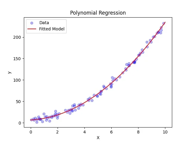
# Plot the data and the fitted model
plt.scatter(X['area'], y, label='Data', alpha=0.3, color='blue')
X_plot_poly = poly_features.transform(X_test)
y_plot = model.predict(X_plot_poly)
plt.plot(X_test, y_plot, label='Fitted Model', color='red')
plt.legend()
plt.xlabel('X')
plt.ylabel('y')
plt.title('Polynomial Regression')
plt.show()Conclusion
Recap of the significance of polynomial regression
Polynomial regression is a powerful and flexible technique for modeling nonlinear relationships between variables.
Furthermore, it can capture complex patterns in data that linear regression may not adequately represent, making it an essential tool in a variety of fields, including engineering, finance, economics, and environmental science.
Future research and advancements in polynomial regression methodology
As machine learning and data science continue to advance, new methodologies and techniques will be developed to further enhance the capabilities of polynomial regression.
Additionally, this may include novel regularization methods, model selection criteria, or computational techniques to improve the efficiency of fitting and predicting with such models.
Final thoughts on the role of polynomial regression in modern machine learning applications
While polynomial regression has its limitations, it remains a valuable method for modeling complex relationships between variables.
So by understanding its strengths and weaknesses and applying it appropriately, researchers and practitioners can continue to benefit from its versatility and interpretability in various real-world applications.