Home » Machine Learning » Anomaly Detection Tensorflow Example

Anomaly Detection Tensorflow Example

In the following example, we’ll look at a demonstration of anomaly detection algorithm using Tensorflow.

Furthermore, we’re going to make an algorithm that can distinguish fraudulent credit card transactions from legitimate ones. Since anomaly detection falls under unsupervised learning category, we’re going to use an autoencoder machine learning model.

Firstly, these types of models work by deconstructing a data sample down to lower dimensional space. And then reconstructing them back again into its original shape.

Therefore, we can train it on legitimate transactions, and when we feed it a fraudulent example, it won’t be able to reconstruct it as perfectly. Thus, setting it apart from the legitimate ones.

Coding anomaly detection algorithm with Tensorflow

First thing we need to do is import all the necessary libraries for importing, visualizing and preprocessing data. Of course, for the machine learning part, we also need the Tensorflow library, so we import that as well.

import pandas as pd
import numpy as np
import tensorflow as tf
import matplotlib.pyplot as plt 
from sklearn.model_selection import train_test_split
from sklearn.preprocessing import Normalizer, MinMaxScaler
from sklearn.pipeline import Pipeline
from kaggle.api.kaggle_api_extended import KaggleApi

Since we’re going to use Kaggle API to download the dataset directly from the script, we need to authenticate connection to it.

# authenticate connection with Kaggle API
api = KaggleApi()
api.authenticate()

After that, we can download the dataset and load it into a pandas dataframe.

# download dataset from https://www.kaggle.com/datasets/mlg-ulb/creditcardfraud
api.dataset_download_files(
    'mlg-ulb/creditcardfraud',
    path='datasets',
    unzip=True
)

# load the dataset into a pandas dataframe
df = pd.read_csv('datasets/creditcard.csv')

Next, we’ll to set some hyperparameters, which we’ll use throughout the whole process. We’re also going to set the seed for random functions, so we can reproduce same results.

# set hyperparameters
RANDOM_SEED = 42
TRAINING_SIZE = 200000
VAL_SPLIT = 0.2
BATCH_SIZE = 256
EPOCHS = 200

# set seed for random values
np.random.seed(RANDOM_SEED)
tf.random.set_seed(RANDOM_SEED)

Now we’re ready to preprocess and prepare our dataset for our model.

Following process includes:

• tweaking the names of columns,
• bringing amount values into logarithmic scale range,
• removing unnecessary columns
• separating fraudulent and legitimate transactions into each own dataframe
• assigning examples into training, validation and testing subsets
• creating a pipeline for data normalization

# process column names
df.columns = map(str.lower, df.columns)
df.rename(columns={'class': 'label'}, inplace=True)

# bring amount values into logarithmic scale
df['log10_amount'] = np.log10(df.amount + 0.00001)

# remove unnecessary columns
df = df.drop(['time', 'amount'], axis=1)

# separate fraudulent and legitimate transactions
fraud = df[df.label == 1]
legit = df[df.label == 0]

# prepare dataset for autoencoder model
legit = legit.sample(frac=1).reset_index(drop=True)
X_train = legit.iloc[:TRAINING_SIZE].drop('label', axis=1)
X_test = legit.iloc[TRAINING_SIZE:].append(fraud).sample(frac=1)

X_train, X_val = train_test_split(
    X_train,
    test_size=VAL_SPLIT,
    random_state=RANDOM_SEED
)

X_test, y_test = X_test.drop('label', axis=1).values, X_test.label.values

print(f"""
    training (rows, cols): {X_train.shape}
    validation (rows, cols): {X_val.shape}
    testing: (rows, cols): {X_test.shape}""")

pipeline = Pipeline([
    ('normalizer', Normalizer()),
    ('scaler', MinMaxScaler())
])

pipeline.fit(X_train)

X_train_fitted = pipeline.transform(X_train)
X_val_fitted = pipeline.transform(X_val)

Next step in this process is to set up the autoencoder model, compile it and train it.

# create autoencoder architecture
input_dim = X_train_fitted.shape[1]

autoencoder = tf.keras.Sequential([
    tf.keras.layers.Dense(input_dim, activation='elu', input_shape=(input_dim,)),
    tf.keras.layers.Dense(16, activation='elu'),
    tf.keras.layers.Dense(8, activation='elu'),
    tf.keras.layers.Dense(4, activation='elu'),
    tf.keras.layers.Dense(2, activation='elu'),
    tf.keras.layers.Dense(4, activation='elu'),
    tf.keras.layers.Dense(8, activation='elu'),
    tf.keras.layers.Dense(16, activation='elu'),
    tf.keras.layers.Dense(input_dim, activation='elu')
])

# compile it and make early stopping and checkpoint save callbacks
autoencoder.compile(
    optimizer='adam',
    loss='mse',
    metrics=['acc']
)

print(autoencoder.summary())

early_stopping = tf.keras.callbacks.EarlyStopping(
    monitor='val_loss',
    min_delta=0.0001,
    patience=10,
    verbose=1,
    mode='min',
    restore_best_weights=True
)

save_model = tf.keras.callbacks.ModelCheckpoint(
    filepath='autoencoder_best_weights.hdf5',
    save_best_only=True,
    monitor='val_loss',
    verbose=0,
    mode='min'
)

# train the model
history = autoencoder.fit(
    X_train_fitted, X_train_fitted,
    shuffle=True,
    epochs=EPOCHS,
    batch_size=BATCH_SIZE,
    callbacks=[early_stopping, save_model],
    validation_data=(X_val_fitted, X_val_fitted)
)

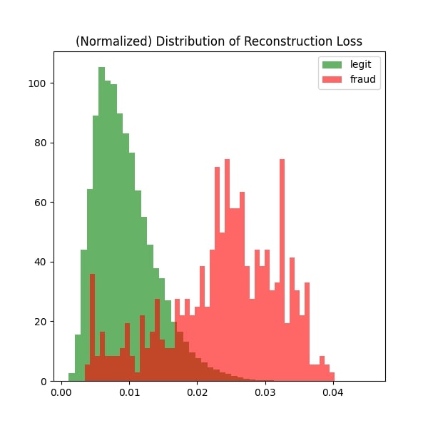
After our model finishes training, we can evaluate it on testing subset and visualize the results.

# evaluate it on test data
X_test_fitted = pipeline.transform(X_test)
eval = autoencoder.predict(X_test_fitted)

mse = np.mean(np.power(X_test_fitted - eval, 2), axis=1)
print(mse)
legit_predicted = mse[y_test == 0]
fraud_predicted = mse[y_test == 1]

# visualize results
fig, ax = plt.subplots(figsize=(6,6))
ax.hist(legit_predicted, bins=50, density=True, label='legit', alpha=.6, color='green')
ax.hist(fraud_predicted, bins=50, density=True, label='fraud', alpha=.6, color='red')
plt.title('(Normalized) Distribution of Reconstruction Loss')
plt.legend()
plt.show()

As we can see, it’s not perfect. However the results show promising signs that with further improvement to the model, we could make it reliable enough for practical deployment.

Conclusion

To summarize, we created a simple autoencoder model for anomaly detection using Tensorflow machine learning library.

I hope this guide helped you gain a better understanding of how to build and implement anomaly detection algorithms.